Creating a simple work program and display it as a Bar chat is relative cheap. This can be done by doing it with Microsoft Excel. However It is very tough to display the critical path and it seems to be impossible to show the logic link between bars. Another disadvantage of this is that it might only practical and applicable to a small scale project that having not more than ten (10) activities. It is due to the complexity of the process in creating the bar chart and it is very time consuming. Below are free step by step guidance to produce a simple work program using Microsoft Excel.
Step 1.
Open the Microsoft Excel Program and create table as picture below (table can be customized according to what information you want to display.

Step 2:
Insert your the task in the task column and task ID in the ID column and arrange it according to level of work or in words it shall be the work breakdown code.
Step 3:
Set the DURATION column by highlighting the column and right click. The dialogue box will appear. from the dialogue box, select "format cell". I should appear like picture below.

After selecting the "format Cells", a dialogue box will appear as below.
 Now Under category, Select Number. I set the decimal point to "0" decimal places. then click OK.
Step 4:
Now start Insert Number of duration. See the following Picture.

Step 5:
In this stage or step 5, for column level as " Start " and " finish", highlight both column, Right click and select " Format cells", a dialogue will appear and under the " Category" select Date and set the " date format". See picture below.


Step 6:
After you select your date format which is shown under the "type" tab. Click "OK". Than Start by inserting the start date as per sequence of work. As a guide you can fill the sequence number base on the ID into the "Predecessor" and "Successor Column". Picture below.

For the "Start", "Finish", "Predecessor" and "Successor" column, If you are familiar with Excel Function or Formula, it is better to use the features since with that Features you can easily create links between cells. Or else you will have to fill and calculate it manually.
Step 7:
Next step is to group task under a major task. To do this, First select "Data Tab". See Picture Below.
 Then, identify which is the major task. Next highlight the "Rows" which represent minor tasks that form the major task. Picture Below
 After Highlighting the minor task, Click on the " Group" Icon under " Data Tab". It will automatically display the Sheet Like picture below.
 The finish product is as picture below.

After you fill in all the data you needed in the table. It is now we can start to create the " Bar Chart".


Still
on the dialogue box, click on the number, then go to the category And choose “
date” and choose the date format type which you want to display on your chart.
After that step, you can choose the alignment tab in the dialogue box to
align the position of your date. See Picture below.


Step 1.
Open the Microsoft Excel Program and create table as picture below (table can be customized according to what information you want to display.
Step 2:
Insert your the task in the task column and task ID in the ID column and arrange it according to level of work or in words it shall be the work breakdown code.
Step 3:
Set the DURATION column by highlighting the column and right click. The dialogue box will appear. from the dialogue box, select "format cell". I should appear like picture below.
After selecting the "format Cells", a dialogue box will appear as below.
Step 4:
Now start Insert Number of duration. See the following Picture.
Step 5:
In this stage or step 5, for column level as " Start " and " finish", highlight both column, Right click and select " Format cells", a dialogue will appear and under the " Category" select Date and set the " date format". See picture below.
Step 6:
After you select your date format which is shown under the "type" tab. Click "OK". Than Start by inserting the start date as per sequence of work. As a guide you can fill the sequence number base on the ID into the "Predecessor" and "Successor Column". Picture below.
For the "Start", "Finish", "Predecessor" and "Successor" column, If you are familiar with Excel Function or Formula, it is better to use the features since with that Features you can easily create links between cells. Or else you will have to fill and calculate it manually.
Step 7:
Next step is to group task under a major task. To do this, First select "Data Tab". See Picture Below.
After you fill in all the data you needed in the table. It is now we can start to create the " Bar Chart".
Step 8
To create the “bar
Chart” , First highlight the Row and column that contained the “ Task”, “Duration”,
“start” and “Finish”. Next, Click on the “Insert tab” , then go to “ bar” then click the icon “ Stacked Bar”. See
picture below.
Once you click on
the icon “ Staked Bar”, a Bar chart will automatically appear in your work
Sheet. It shall look like the picture below.
Step 9:
Next, in the Start
and finish Column, Identified the Earliest date to start work. Right Click on
that cell, then click “ format cell”. A dialogue box like below will appear.
Inside the dialogue
box, under category, click on “number”. Once you click on the “number”, under
the sample, you will see a set of number. In this example the number is 41703.00. This number is actually represent
the date of 05/03/2014. See picture below. Write down this number on a piece of
paper. After you done with this step, Click the “cancel” tab. The dialogue box
will close by itself. Next, do the same thing to the last date which you are
going to complete your work or task. You will need those number to customized the
date axis range on your chart later on.
Step 10.
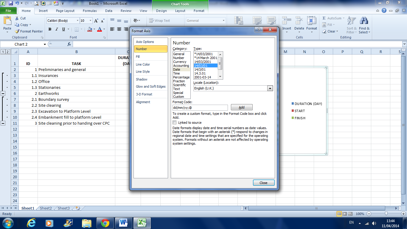
Right Click on the “X”
axis and then Click “ format axis”. Refer to picture below.
After you click the
“format axis” a dialogue box will appear as below.
Inside the axis
option check the minimum value to fixed and insert the number for start date
which you write down earlier in step 9.
Do the same for maximum Value but inset the number which will represent the
last completion date of the work.
One you done with
it, click “Close”. Your Chart Should appear like this.
Step 11
Right click on the “Y”
Axis and click Format Axis. A dialogue box like below will appear.
Inside this dialogue
box, look for the “ Category in reverse order”.
“Checked “ the box and next Close the dialogue. Your chart should be
displayed as below.
Step 12
In the Chart, Right
click in between two bars. Then Click “select data” . See picture below.
One you had click
on the “select data” a dialogue box as below will appear.
Click on the “Duration”
follow by clicking on the “move down” button. This will change the position of
your “Duration”. Once you done with
that, Click “ OK” tab. It will close the Dialogue box. This action will make
your Chart look as this following picture.
Step 13
Still
on the chart. Right Click on any of the green bar.
Then, click on the “fill
colour” icon. Picture below.
Choose the “no fill”
. Your chart should be as follows.
Repeat this step 13
but now do the same for the bar that is “red” in colour.The end product for
this step shall be displayed as below.
Step 14
Now identify the “Critical
Path” and recoloured it into red. You should have a Bar chart as below.
Step 15
If you want to show
both “ Start” and “ Finish” date, Click on the bars that represent the “Start”
bar
(already recoloured with no fill in step 13),then click the “ Add data
level’.
Your chart will
look like this.
Now the start date had been
inserted. However the date been displayed and overlap with other information. We
don’t want this display. Hence we need to re format the “ X “ axis. To Do That
we need to change the Minimum Value and the maximum value of “X” Axis. See the
pictures below. For Minimum value,
entered value that is less than 41703 and for Maximum Value entered number
greater than 41848.
Next, for the “finish
date” do the same procedure as what had been done for “ Start Date” but for
“ the Finish date” click on the “finish Bar” which had been recoloured
earlier with “No Fill”. Your end product shall be displayed as follow.
Basically, Your
work program created with Microsoft Excel is now completed. However for a better presentation of Your Bar Chart, you Can present it as Chart on its
own or you can rearrange is such a way
to be display with full description.
a) Bar Chart
represent the work program on its own.
b) Work program
with full description.
Congratulation. You just finish creating the work program by using Microsoft Excel.